Causal Inference: Notes from a Cornell PhD-Level Econometrics Course (2)

Starter notes from a PhD-level econometrics course on how to think clearly about causality in observational data.

Course taken: Cornell PAM 6090 Time taken: Fall 2021

This article is a continuation of the first econometrics class note: Causal Inference: Notes from a Cornell PhD-Level Econometrics Course (1)

What We Will Cover

• What are the assumptions of OLS?

• When does OLS really fail?

• How do we fix OLS failure?

• Causal Identification Strategies

Section 1: Assumptions of OLS

OLS regressions form the building blocks of econometrics.

Based on the building blocks of OLS—and by relaxing certain assumptions—several different models have been developed, such as GLMs (generalized linear models), general linear models, heteroskedastic models, multilevel regression models, etc.

The necessary OLS assumptions used to derive the OLS estimators in linear regression models are discussed below.

A1: Linearity in Parameters

The model is linear in β. Variables can be transformed, but coefficients must enter linearly.

For example:

\(y = \beta_0 + \beta_1^2 x + u\)

Here, β₁ is squared → not linear in parameters.

A2: Random Sampling of Observations

Observations are independently and identically drawn from the population.

A3: No Perfect Multicollinearity

No regressor is an exact linear combination of others.

For example, X_n cannot be expressed as X_1 + X_2 + …

A4: Zero Conditional Mean (Exogeneity)

\(E[\text{error} \mid X] = 0\)

The distribution of error terms has zero mean and does not depend on the independent variables. Thus, there must be no relationship between the X’s and the error term.

This is the most important assumption. It gives unbiasedness and consistency.

A5: Homoskedasticity (for BLUE: Best Linear Unbiased Estimator)

The error terms in the regression should all have the same variance.

If this variance is not constant (i.e., it depends on X’s), then the linear regression model has heteroskedastic errors and is likely to give incorrect standard errors.

Additionally, the assumption of no autocorrelation states that the error terms of different observations should not be correlated with each other.

For example, in time series data (e.g., yearly unemployment rates), the regression is likely to suffer from autocorrelation because unemployment next year depends on unemployment this year. Hence, error terms across observations may be correlated.

A6: Normality (Only for Exact Small-Sample Inference)

This assumption states that the errors are normally distributed, conditional on the independent variables.

Normality is not required for the validity of OLS. However, it becomes important when defining additional finite-sample properties.

Note:

• Only the error terms need to be normally distributed.

• The dependent variable Y does not need to be normally distributed.

This assumption is only needed if:

• Your sample is small, and

• You want exact hypothesis tests.

Compact Summary

• Zero conditional mean → Unbiased + Consistent

• Add homoskedasticity → BLUE

• Large sample + finite variance → Asymptotic normality

• Normal errors → Exact small-sample inference

Section 2: When Does OLS Really Fail?

The true killer is endogeneity:

\(E[\text{error} \mid X] \neq 0\)

This destroys unbiasedness and consistency. Everything else mainly affects efficiency or inference.

What Happens When Assumptions Fail?

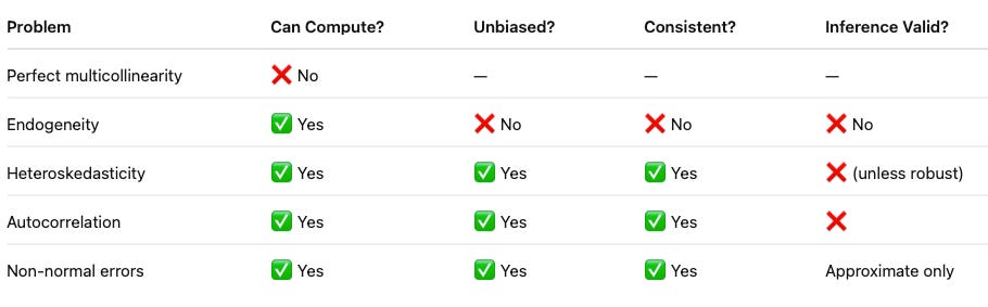
OLS Fails Fundamentally When Regressors Are Correlated with the Error Term.

Examples:

1. Omitted variables ( Example: Education and Salary. You study whether more education increases salary. But you forget to include ability. In real life: Smarter or more motivated people tend to get more education. Those same people also earn higher salaries. )

2. Reverse causality ( Example: Health and Income. You study whether higher income improves health. But in real life: Healthy people are able to work more. They earn higher income. Now income and health influence each other. Your regression can’t tell which direction the effect runs. You might conclude income improves health, when actually good health helps people earn more.)

3. Measurement error in X ( Example: Exercise and Weight Loss. You study whether exercise reduces weight. But exercise is self-reported. People overestimate or misreport how much they exercise. So your “exercise” variable is noisy. Reported Exercise = True Exercise + Measurement Error. And the regression error now also contains that measurement error. So part of the regressor literally shows up inside the error term.

Section 3: How to Fix OLS Failure

Almost all causal methods try to solve the same core problem:

The regressor is correlated with the error term.

They fix it by:

1. Removing confounders (controls / fixed effects)

2. Isolating exogenous variation (IV)

3. Creating exogenous variation (RCT)

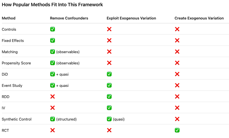
All of these methods attempt to restore the key condition:

\(E[\text{error} \mid X] = 0 \)

They simply do it in different ways.

Section 4: Causal Identification Strategies

Many scholars have written extensively about this topic. It is well documented in books such as:

• Mostly Harmless Econometrics

• Causal Inference: The Mixtape

So, I will not go into the technical details of the identification strategies in this article. Instead, I will provide a link to my notes for reference. In addition to the notes, I have summarized papers that apply each identification method, primarily in service-related research.

Causal Inference in Service Research

To cite:

Wang, Frances. 2025. Causal Inference in Service Research. PhD diss., Cornell University.

Please feel free to share any suggestions for future topics or any thoughts you may have ! :))) Happy lunar new year! Welcome the year of horse 🐎～